24. Linear regressions in R
The linear regression is the workhorse model in science. Today I’ll teach you how to use it in R.
Make some random data
To get started, let’s make a linear relation between two variables, x and y. To do that, we’ll use the rnorm function, which generates random numbers from a normal distribution.
The code below generates 1000 random numbers from a normal distribution with a mean of 0 and standard deviation of 1. We’ll call this batch of numbers x:
x = rnorm( n = 1000, mean = 0, sd = 1 )
Next, let’s generate some statistical noise. Like x, our noise will be random numbers from a normal distribution. But we’ll make the standard deviation smaller than in x. Let’s make it sd = 0.2:
noise = rnorm( n = 1000, mean = 0, sd = 0.2 )
Finally, let’s make a linear relation. We’ll define the variable y as:
y = x + noise
Plot your data first!
Looking ahead, we’re going to fit a linear regression to our x-y data. But before we do that, it’s always best to plot the data to see what it looks like. Let’s do that now:
plot(x, y)
The result looks like this — a nice linear relation between x and y:
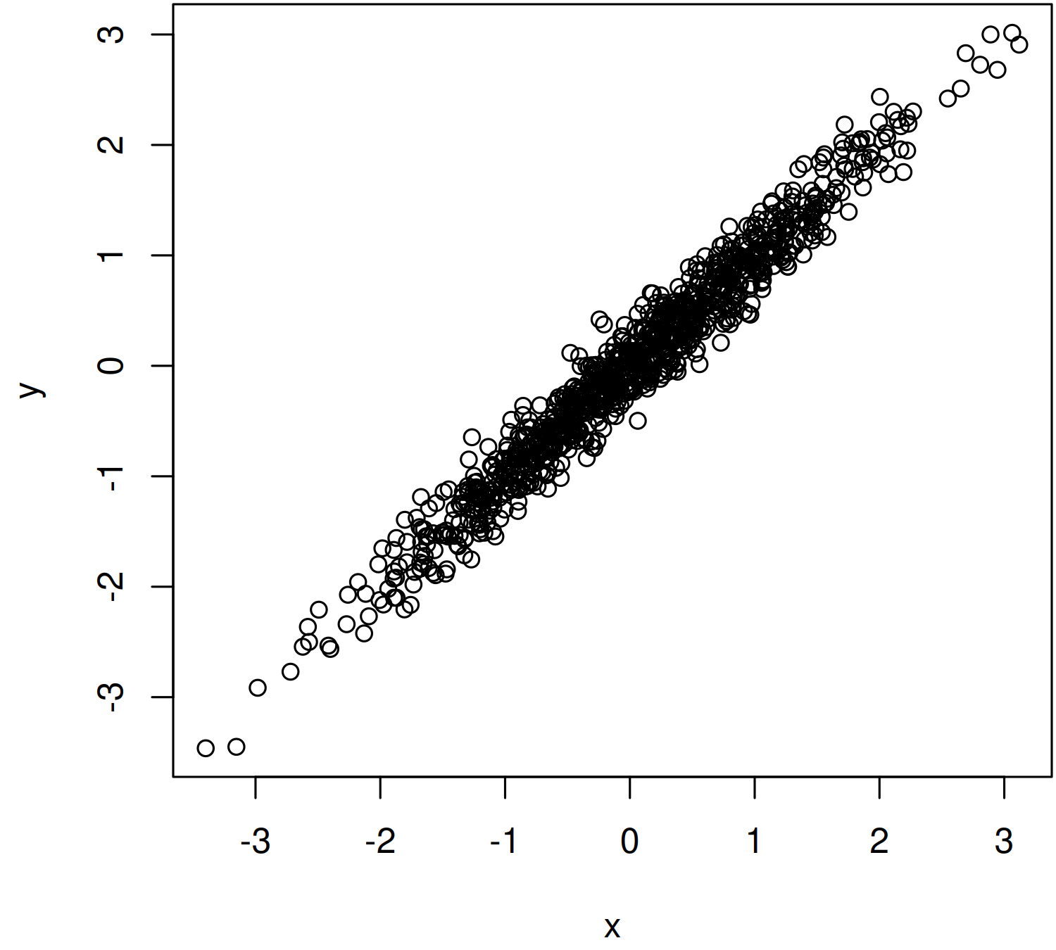
Warning: if you plot your data and find that the trend is curved, stop now. It’s silly to fit a linear model to curvy data. You’ll need to do something more sophisticated, which I’ll discuss another time.
Correlation
Alright, we’ve got a linear relation. Before we run a regression, let’s start with its simpler cousin, the correlation.
To get the correlation coefficient between two sets of data, we use the cor function:
cor(x, y)
It will spit back the correlation coefficient between x and y. As expected, it’s high:
> cor(x, y)
[1] 0.9797063
For some context, the correlation coefficient is a number that varies from -1 to 1. It’s often given the symbol r:
- r = 0: no correlation
- r = 1: a perfect positive correlation
- r = -1: a perfect negative correlation
So our x-y relation has a correlation coefficient of r = 0.98 — a strong relation.
Linear regression
Now to our more complicated friend, the linear regression. To run a regression in R, we use the lm function. Here’s what it looks like:
lm( y ~ x )
Some notes. Yes, you need to put the dependent variable (here y) before the independent variable (here x). And if you’re wondering, the ~ symbol is code for ‘related to’.
Let’s look at the output of this code:
> lm( y ~ x )

Call:
lm(formula = y ~ x)

Coefficients:
(Intercept)            x
   0.009812     1.005313
Right away, you can see that it’s more complicated that the output of the correlation function. Here’s what it means.
First, R dumps back the formula that you gave it:
Call:
lm(formula = y ~ x)
Next, R tells you the coefficients of the linear regression.
Coefficients:
(Intercept)            x
   0.009812     1.005313
To make sense of these numbers, let’s review some high school math. The equation for a line is often taught as:
y = mx + b
Here m is the slope and b is the y intercept. To confuse you a bit, statisticians usually flip the order of the equation like this;
y = b + mx
Thinking like a statistician, R dumps the coefficients in this latter order. So the intercept (b) is 0.0098. And the slope (m) is 1.005. So our model is;
y = 0.0098 + 1.005 x
Now we can see what our noise did. Without it, we’d have a perfect linear relation, y = x. But the noise fudges things up, adding a non-zero intercept and making the slope differ slightly from 1.
Accessing the full regression menu
To recap, if we put lm( y ~ x) into the terminal, R will dump the coefficients of the regression. But under the hood, R can give us much more detail.
To see these details, we need to save our regression as a variable. Let’s call it model:
model = lm( y ~ x )
To get the gory details about our model, we can use the summary function:
summary( model )
We’ll get a data dump that looks like this:
Call:
lm(formula = y ~ x)

Residuals:
     Min       1Q   Median       3Q      Max
-0.72652 -0.13974 -0.00039  0.13968  0.75094

Coefficients:
            Estimate Std. Error t value Pr(>|t|)
(Intercept) 0.009812   0.006531   1.502    0.133
x           1.005313   0.006511 154.412   <2e-16 ***
---
Signif. codes:  0 ‘***’ 0.001 ‘**’ 0.01 ‘*’ 0.05 ‘.’ 0.1 ‘ ’ 1

Residual standard error: 0.2065 on 998 degrees of freedom
Multiple R-squared:  0.9598,	Adjusted R-squared:  0.9598
F-statistic: 2.384e+04 on 1 and 998 DF,  p-value: < 2.2e-16
There’s a confusing amount of information here, so let’s wade through it.
First, R gives us a summary of the regression ‘residuals’. These are the distances between the y values in our data and the y values in our model.
Residuals:
     Min       1Q   Median       3Q      Max
-0.72652 -0.13974 -0.00039  0.13968  0.75094
Next, R dumps the coefficients of the linear model. The actual estimates are in the Estimate column. Next to these values, we get a bunch of statistics that I won’t wade through here.
Coefficients:
            Estimate Std. Error t value Pr(>|t|)
(Intercept) 0.009812   0.006531   1.502    0.133
x           1.005313   0.006511 154.412   <2e-16 ***
---
Signif. codes:  0 ‘***’ 0.001 ‘**’ 0.01 ‘*’ 0.05 ‘.’ 0.1 ‘ ’ 1
Finally, we get a summary of the regression fit, the most important of which is the R-squared value.
Multiple R-squared: 0.9598, Adjusted R-squared: 0.9598
Getting coefficients and the R-squared value
Having confused you with R’s data dump, let’s make things simpler.
When I run a regression, I typically want to save the regression coefficients. To get them, we first save our regression (here as model). Then we extract the model coefficients (the y-intercept and slope) using the coef function:
model = lm( y ~ x )
model_coefficients = coef(model)
Let’s have a look at them:
> model_coefficients
(Intercept)           x
0.009811796 1.005312922
Yep, still the same as before.
Now let’s extract the R-squared value. To do that, we use this code:
summary(model)$r.squared
I get back an R-squared of about 0.96 — nice and high:
> summary(model)$r.squared
[1] 0.9598244
But wait, what does an R-squared value mean? Well, in simple terms the R-squared tells us the portion of variation in y that is explained by our linear model. So in this example, a linear model between y and x explains 96% of the variation in y.
Some homework
To get comfortable with linear regressions, here’s some homework.
First, try adjusting the standard deviation in the noise distribution. Here, for example, I’ve increased the noise to have sd = 0.6. See how that affects the regression.
x = rnorm( n = 1000, mean = 0, sd = 1)
noise = rnorm( n = 1000, mean = 0, sd = 0.6 )
y = x + noise
You can also change the slope of the relation like this:
y = 3*x + noise
You might also try varying the sample size. To do that, change the n value in the rnorm function. Here’s a sample size of 10:
x = rnorm( n = 10, mean = 0, sd = 1)
noise = rnorm( n = 10, mean = 0, sd = 0.6 )
y = x + noise
See what you find!